
Skeptical MedicineJohn Byrne, M.D
|
Bayesian Statistics
In the What is Science section, we learned a little bit about Bayesian methods for assessing the probability of a hypothesis. We saw that the probability of a hypothesis in light of new evidence is proportional to its prior probability times the strength of the new evidence.
Bayesian statistics allow one to make an estimate about the likelihood of a claim and then update these estimates as new evidence becomes available.
In non-mathematical terms, Baye’s Theorem can be expressed like this:
The probability of a claim (given the currently available data) is proportional to its probability before the new data multiplied by the strength of the new data. Thus, we put new data into perspective with our prior understanding.
This form of statistical methodology stands in contrast to traditional statistics called frequentist probability, whereby the probability of an event is determined only after counting its frequency after collecting a body of data. In Frequentism, conclusions tend to be fairly binary (we either reject the null hypothesis in favor of the pet hypothesis, or we do not).
Statistical significance is said to be met if the p value is below a certain limit, usually set as p < 0.05).
Current medical studies tend to utilize frequentist probability. As discussed in the EBM vs. SBM section, such statistics only count frequencies of events to determine ‘significance’. Plausibility of the hypothesis in question does not really play much of a role.
With Bayesian statistics, plausibility determines the starting point for determining a claims probability. Thus, we have the SBM call for using Bayes especially when dealing with highly implausible claims.
History
History was sluggish and frankly unkind to Baye’s Theorem. Sharon Mcgrayne’s book, The Theory That Would Not Die, describes a remarkable evolution of such a simple idea.
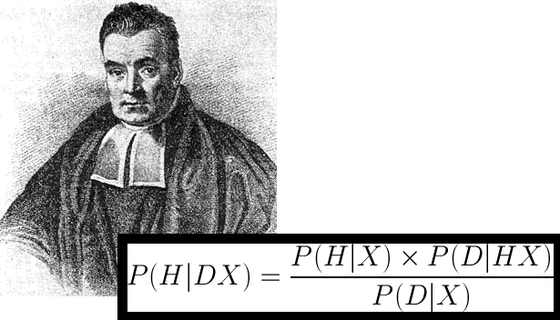
Thomas Bayes (1701 – 1761) was a British mathematician and a minister. He is credited for describing a process for adjusting and updating the likelihood of an event based on data — as the data is generated. Remember, in frequentist statistics, probabilities are determined only after all of the data is collected. He did not publish this as a mathematical theorem, but rather described the basic idea in a posthumous publication, “An Essay towards solving a Problem in the Doctrine of Chances“.
In 1814, the French mathematician, astronomer and statistician Pierre-Simon Laplace published Essai philosophique sur les probabilités. Here, he described mathematically the same idea that Bayes had described earlier.
Until recently, statisticians have shunned Bayesian methodology due to the fact that it begins with uncertainty (and corrects with each new observation toward the likely truth). In her book, Mcgrayne describes those that discovered the power of Bayesian statistics over the twentieth century. Perhaps the most notable was Alan Turing. During World War II, Turning used Bayesian methodology and early computers to decipher Nazi u-boat codes. Historians acknowledge that Turing’s work likely helped turn the tide of the war in the Allies’ favor. His work and methods, however, were classified by Winston Churchill after the war. The world and statisticians would not know of the success until decades later.
In the era of modern computers, Bayesian methodology has been rediscovered and updated. Prior probabilities are now calculated from our large body of prior scientific knowledge, specialized expertise or by recently developed statistical techniques. However, there is still some inherent subjectivity to the starting point.
Prior Probability
|
|

Ideas and theories start out with a baseline probability of being true based on previously established knowledge. Bayesians call this the prior probability, or just “the prior”. The prior can be somewhat subjective, as it is sometimes an unknown quantity based on limited data and the biases of the person assigning the value. It is a measure of belief that the claim is true. Bayes’ allows multiple hypotheses to be combined and ranked by probability. The prior is usually written as P(H). Each hypothesis for a given problem is distinguished with a number (H1, H2, etc). The “null hypothesis” is notated as Ho.
Skeptics often employ Occam’s Razor when assigning relative values to priors. Before new data is collected or observed, we can rank competing hypotheses according to the number of assumptions required by each one. Hypotheses that only incorporate established knowledge are given higher probabilities than those that either require us to accept unknowns or to reject established knowledge.
For instance, explanations that suggest a violation of physics (eg. homeopathy) or the presence of an unknown vital force (eg. acupuncture, reiki, chiropractic) have more built-in assumptions than explanations that only require acceptance of known processes (eg. phychology, statistical trends, natural history of disease). Plausible explanations that incorporate the fewest unknowns and assumptions are ranked with higher priors than those with such assumptions. The more assumptions made lead to lower the ranking of prior probability. Also, the more violations of established knowledge, the lower the prior probability.
When determining the prior probability for events that have a known background rate, we may use this background rate (or “base rate”) as our prior. When determining the likelihood of a disease in a patient, we can begin with the base rate of the disease in the community in which the patient is a member. If a patient belongs to a community that has a base rate of HIV infection of 1%, then we use 1% as our prior probability when determining the likelihood of the patient’s status (even before gathering any information about the patient).
It must be acknowledged that many will find explanations with lower priors to be appealing due to biases, beliefs and world views. We may find comfort in explanations that appeal to unseen forces, new-age ideas and dogma. Appealing as they may be, priors should be assigned with Occam’s Razor in mind.
New Data, Priors and Posterior Probability
The next step in the Bayesian approach involves the consideration of new data obtained through experimentation or observation. We must ask, ‘what is the probability of obtaining a set of data if the hypothesis were true?” In other words, how much does the data support the given hypothesis. This is commonly written as P(D/H), or the probability of the data given the hypothesis.
Here we assign a probability that the new data could be accounted for by the hypothesis in question. Studies are generally designed to test a given hypothesis. It is here that we must account for the strength of the new evidence based on the quality of the study and the magnitude of the results.
Study quality was examined in the section on Scientific Studies in Medicine. Larger studies are typically more powerful than smaller ones. Randomized, double-blinded controlled trials typically are better than observational studies, etc. Results that are unambiguously positive lend more support to a hypothesis than those that barely reach statistical significance.
In Bayes’, we update a the probability of a hypothesis by multiplying the prior probability with the strength of the new data. The new, updated probability is called the posterior probability, or just ‘the posterior’. However, there is a denominator in the calculation. This is the sum total of probabilities of all possible relevant hypotheses. This should be considered to be a constant that, if all hypothesis are truly accounted for are summed, should equal 1. (see below).
The posterior then becomes the new prior and the process may repeat. In other words, the probability of an idea is updated in light of new information and thus should become closer to the truth. The posterior may be higher or lower than the prior and closer to the truth (one may consider “the Truth with a capital T” to be approachable, but ultimately unknowable.)
One can see how this method complies with both Occam’s Razor and the Extraordinary Claims rule, which states, “extraordinary claims require extraordinary evidence.” Occam’s Razor helps to define just how extraordinary a claim is. Bayes’ rule simply helps us to rank hypotheses with these concepts.
Bayes’ in Everyday Medicine
Let’s consider how we can put Bayes’ Theorem to practical use in everyday medical decision making.
Let’s say that a disease is known to have a prevalence of 1 out of every 1000 people in a given population. This gives us our “prior”. (Note – this number is obtained through frequentist statistics. Sometimes the prior probability can be known, other times it comes from an educated guess.)
Let’s also say that we have a test for the disease that is very sensitive, but has an inherent false positive rate of 10%.
Now, we need to use the test on 1000 individuals to determine if they have the disease. The pre-test probability that any one of the individuals has the disease is 1/1000, or .001.
When we test 1000 people, we may find (on average) the 1 person in 1000 that has the disease. But we also find 100 people who test positive but do not have the disease (10% false positive x 1000 people = 100 false positives).
So, we may expect on average to find 101 people that test positive out of the 1000 people tested (1 true positive and 100 false positives). Therefore, of these 101 suspects, each of them only have a 1/101 chance of having the disease. The denominator, 101, represents the sum of our 2 possible hypotheses (101 positive tests = true positives and false positives). The perspective that Bayesian analysis gives us allows us to make better sense of data.
Without understanding that we need to combine the new data with the prior probability, a clinician may tend to raise an unwarranted amount of fear in these 101 patients even though it is likely that only 1 of them has the disease. Without the Bayesian perspective, these 101 people will likely all become convinced that they have the disease.
This exercise demonstrates how we gain a much clearer perspective about test results by combining prior knowledge with new data and updating our position. It demonstrates how we arrive at the positive predictive value of a test. We can similarly determine the predictive value of a test.
Modern Formulation
Bayes’ Theorem is formally notated as:
P(H/D) = P(D/H) x P(H)
P(D)
where…
P(H/D) is the probability of the hypothesis (H) given the data (D),
P(D/H) is the probability of the data (D) given the hypothesis (H),
P(H) is the probability of the Hypothesis prior to the new data (also called the “prior probability” or just the “prior”), and
P(D) is the probability of obtaining the data (D).
The P(D) is the sum of all of the probabilities of obtaining the data for each hypothesis. In hypothesis testing, it can be expressed as the sum of the probabilities of obtaining the data (D) given the hypothesis (H) and the null hypothesis (Ho). This is notated as:
P(D) = P(D/H) x P(H) + P(D/Ho) x P(Ho)
So, we can then write Bayes’ Theorem as:
![]()
Applying Bayesian Methods
Putting these last parts together, we can see some of the true power of Baye’s Theorem. Let’s put Bayes’ in terms of commonly used statistical values (p value, prevalence, sensitivity and specificity).
In frequentist statistics, the highly touted p-value is really the probability of obtaining the data if the null hypothesis were true. In other words,
p-value = P(D/Ho).
Also, we can express the p-value as the probability of obtaining a false negative result. In other words, p-value = (1-specificity).
The prevalence of a condition is its frequency within a population. Therefore, the probability of it not being present is therefore 1 – prevalence. This essentially is the same as saying the probability of the null hypothesis. In other words,
(1 – Prevalence) = P(Ho).
By combining our previous knowledge about a condition (prevalence), and the frequentist parameters of our tests (sensitivity, specificity), we can do some Bayesian analysis, just as we did in the exercise above.
![]()
where PPV is the “Positive Predictive Value“.
Knowledgeable clinicians can use the “Positive Predictive Value” and “Negative Predictive Value” of tests and procedures to make better decisions.
Bayes Factor
This is the ratio of the probabilities of the data in light of the hypothesis (H) and the null hypothesis (Ho).
Bayes Factor = P(D/H)
P(D/Ho)
![]()
This is often used synonymously with the Likelihood Ratio.
The Bayes Factor tells us about the data and how useful it is given the hypothesis being tested.
If the Bayes Factor is 1, then the data would be useless. In other words, data obtained would be equally consistent with H and Ho.
If Bayes Factor is 1 to 2, then the data would be slightly interesting, but likely does not mean a big difference between H and Ho.
If Bayes Factor is 2 to 5, then the data would represent a mild difference between H and Ho.
If Bayes Factor is 5 to 10, then the data would represent a moderate difference between H and Ho. If Bayes Factor is over 10, then the data would represent a large difference between H and Ho.
Bayesians vs Frequentists (SBM vs EBM Revisited)
Medical science is currently evaluated mainly with frequentist statistics. Individual studies and meta-studies are look evaluate data from the prospective of the p-value. To a Bayesian, the p-value is really the probability of the data given the null hypothesis, or P(D/Ho). If the p-value is less than 0.05, we traditionally say the the data is “statistically significant” and we then reject the null hypothesis.
Frequentists have complained that Bayes’ uses subjective values for initial priors (although, modern techniques can be used to reduce the subjectivity). However, the traditional cut off for statistical significance of p < 0.05 is also somewhat subjective. Some studies produce results with a p-value of 0.04. Are these results more significant than those with a p- value of 0.06? Frequentist statistics can lead to a binary mode of thinking. Significant or not significant. Reject or accept.
Typically, studies with a p-value close to 0.05 are labeled ‘inconclusive’ and more studies are called for. The modern world of Evidence Based Medicine tends to operate on frequentist statistics. This is generally fine when analyzing claims with reasonable plausibility. When analyzing low probability claims with respect only to the p-value, we may miss the forest through the trees.
In Bayesian statistics, the p-value is only one part of the denominator. The “prior” is in the numerator and holds a major role in the calculation of the posterior. Therefore, when evaluating claims with low prior probabilities (“extraordinary claims”), Bayesian methodology automatically puts such claims in perspective. Thus, “Science Based Medicine” (SBM) takes a Bayesian approach to extraordinary claims. Bayesians and SBM proponents tend to talk in terms of low and high probability, rather than rejecting or accepting a hypothesis based on the p-value (see EBM vs SBM).
More Bayes in Everyday Life — “21”
Many experienced gamblers employ Bayes’ Theorem everyday in casinos. Blackjack, or “21”, is a game that lends itself perfectly to Bayesian methodology. Unlike roulette, craps or slot machines, 21 is not as subject to the “gambler’s fallacy” in that the odds of the next hand do not reset each time. There are a finite number of cards, and a known number of “high” and “low” cards. The cards are not reshuffled with each hand and not until all of the cards have been dealt (in casinos, a card shoe usually contains 4 decks). Each player only plays against the dealer, who has a slight, inherent advantage. It is generally known that low cards work to the dealer’s advantage, whereas high cards work to the player’s.
Smart gamblers have developed systems of ‘card counting‘. They assign a +1 value to low cards (2’s through 6’s), 0 value to middle cards (7’s, 8’s and 9’s) and -1 value to high cards (10’s through Aces). When each card is dealt and ultimately revealed, the card counter makes a mental addition or subtraction (+1 or -1). With each hand, the card counter calculates a new tally based on the cards already dealt. Tallies that are strongly positive mean that there are more high cards left in the shoe than low cards. This gives the player the advantage and a signal to start placing bigger bets. Values that are strongly negative mean that there are more low cards left, which gives the dealer the advantage.
Prior to any cards being dealt, the tally is 0. This is akin to the initial “prior” in a Bayesian analysis. The card counter then updates this prior probability in light of new data with each hand (tally from the cards that have been dealt). This is all done to determine the probabilities of 3 competing hypotheses (H1 = win, H2 = lose, H3 = break even). Without even realizing it, professional Blackjack players are natural Bayesians.
The 2008 movie, “21” was loosely based on a group of MIT students who used this technique to win big in Las Vegas (they were eventually banned from the casinos). One of the real-life players discussed the technique to promote the movie, as seen here.
Conclusion
By combining the Bayes Factor with the Prior Probability of a hypothesis, we get a very clear picture of just how probable a hypothesis is in light of new data. In this way, the probability of an idea being true may always be adjusted in light of its prior probability and new data. We may have a better understanding over time, in light of multiple studies, of the truth of an idea.
Currently, we tend to judge the significance of a study on the p-value. As more studies are done, each study basically starts from scratch and comes up with new p-values. Each study may have biases and methodological flaws. Commonly, multiple studies – with their flaws – are combined into a meta-analysis to make one big study with its own p-value. This works fairly well for ideas that have high prior probabilities (in other words, the ideas are plausible in light of prior scientific knowledge). However, skeptical doctors are also concerned with ideas and claims that have low prior probabilities.
For ideas with low prior probabilities, it may be more useful to use a Bayesian approach (using the Bayes Factor and prior probability to determine a new probability of an idea in light of new data). Instead of combining data from multiple studies into a meta-analysis, each study should add to the probability. The Bayes Factor of the study would determine the value of the data produced by the study. Poor studies would have low Bayes Factors, and contribute less to the big picture than would good studies.
John Byrne, M.D.
References and Links
“The Theory That Would Not Die: How Bayes’ Rule Cracked the …” 2012.
<http://www.amazon.com/dp/0300188226>
“An Essay towards solving a Problem in the Doctrine of Chances …” 2011.
<http://en.wikipedia.org/wiki/An_Essay_towards_solving_a_Problem_in_the_Doctrine_of_Chances> “Essai philosophique sur les probabilités – Cambridge Books Online …” 2011.
<http://ebooks.cambridge.org/ebook.jsf?bid=CBO9780511693182> “Alan Turing – Wikipedia, the free encyclopedia.” 2003.
<http://en.wikipedia.org/wiki/Alan_Turing>
“Science-Based Medicine » Prior Probability: The Dirty Little Secret of …” 2011.
<http://www.sciencebasedmedicine.org/index.php/prior-probability-the-dirty-little-secret-of-evidence-based-alternative-medicine-2/>
“The Bayesian Trap”, Veritasium YouTube Channelhttps://www.youtube.com/watch?v=R13BD8qKeTg&t=94s